visualize
Noelle Helder
6/28/2021
3.1 Read Data
# libraries
library(here)
## Warning: package 'here' was built under R version 4.0.3## here() starts at C:/Users/noell/Documents/2021_NOAA_OER/r3-exerciseslibrary(readr)
library(DT)
library(tidyverse)
# variables
url_ac <- "https://oceanview.pfeg.noaa.gov/erddap/tabledap/cciea_AC.csv"
# 'here' prefixes this to give me the full path. this helps make this really portable. If someone else clones this file to their machine, this ensures that it will work when they run this.
# here looks for the project file (.Rproj) and then sets the project as the root and updates the paths accordingly. It will work regardless of where you move it when you reference with here.
csv_ac <- here("data/cciea_AC.csv")
# read data
d_ac <- read_csv(url_ac, col_names = F, skip = 2) # column names = false, then skip 2 lines of the header## Parsed with column specification:
## cols(
## .default = col_double(),
## X1 = col_datetime(format = "")
## )## See spec(...) for full column specifications.names(d_ac) <- names(read_csv(url_ac))## Parsed with column specification:
## cols(
## .default = col_character()
## )
## See spec(...) for full column specifications.# show data
datatable(d_ac)3.2 Plot statically with ggplot2
3.2.1 Simple line plot + geom_line()
# subset data
d_coast <- d_ac %>%
  # select columns
  select(time, total_fisheries_revenue_coastwide) %>%
  # filter rows
  filter(!is.na(total_fisheries_revenue_coastwide))
datatable(d_coast)
# ggplot object
p_coast <- d_coast %>%
# setup aesthetics
ggplot(aes(x = time,
y = total_fisheries_revenue_coastwide)) +
# add geometry
geom_line()
# show plot
p_coast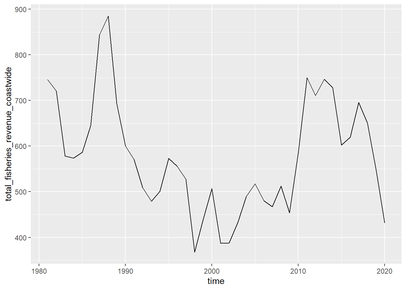
# add trendlines
p_coast + geom_smooth(method="loess")
## `geom_smooth()` using formula 'y ~ x'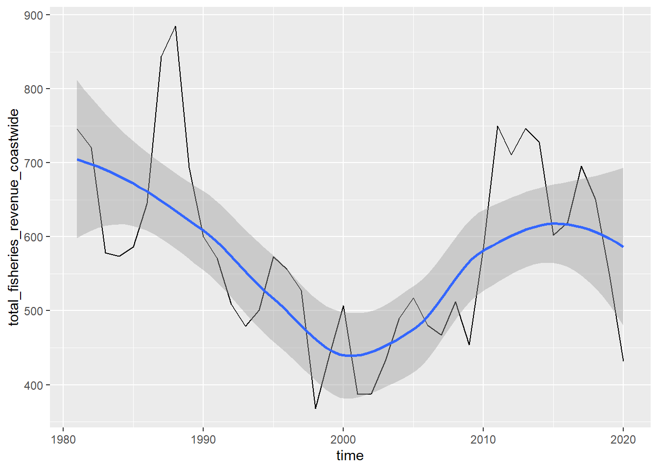
3.2.3 Plot distribution
d_coast %>%
  # setup aesthetics
  ggplot(aes(x = total_fisheries_revenue_coastwide)) +
  # add geometry
  geom_histogram(binwidth= 100)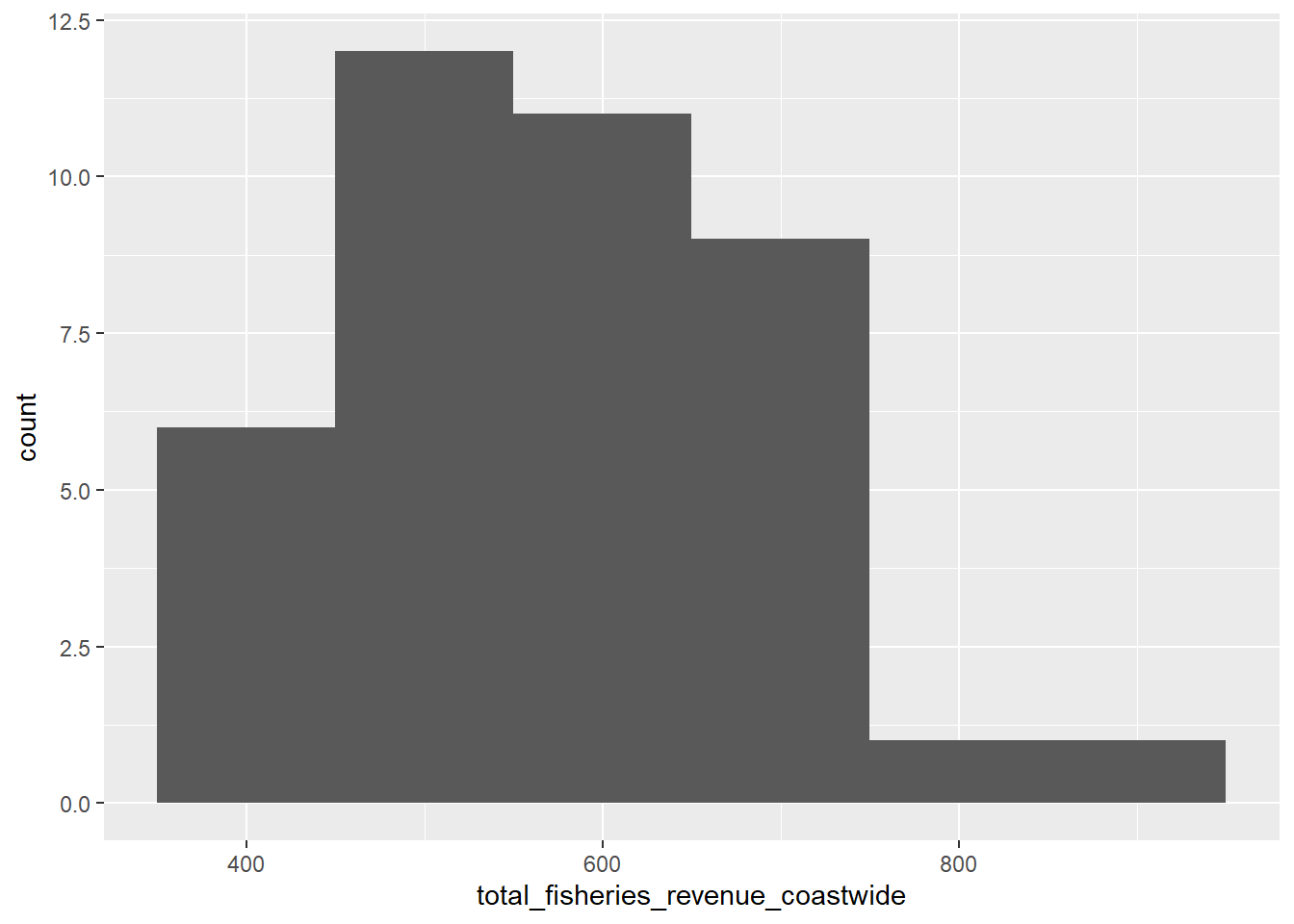
Series line plot by region
library(stringr) # to manipulate strings
library(tidyr) # to pivot data from wide to long

d_rgn <- d_ac %>%
  # select columns
  select(
    time,
    starts_with("total_fisheries_revenue")) %>%
  # exclude column that we've already plotted. left with CA, OR, WA
  select(-total_fisheries_revenue_coastwide) %>%
  # pivot longer: -time means use all of the other columns but keep time because each observation is      unique by time
  pivot_longer(-time) %>%
  # mutate region by stripping other
  mutate(
    region = name %>%
      str_replace("total_fisheries_revenue_", "") %>% # get rid of the prefix and replace it  nothing
      str_to_upper()) %>% # make it uppercase
  # filter for not NA
  filter(!is.na(value)) %>% # filter out things in the 'value' column that are NaNs
  # select columns
  select(time, region, value)

# create plot object
p_rgn <- ggplot(
  d_rgn,
  # aesthetics
  aes(
    x     = time,
    y     = value,
    group = region,
    color = region)) +
  # geometry
  geom_line()

# show plot
p_rgn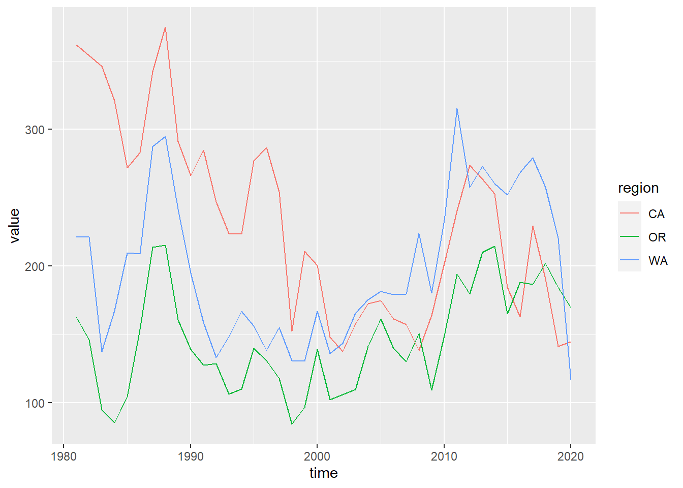
# update labels with + labs()
p_rgn <- p_rgn +
  labs(
    title  = "Fisheries Revenue",
    x      = "Year",
    y      = "Millions $ (year 2015)",
    color  = "Region")
p_rgn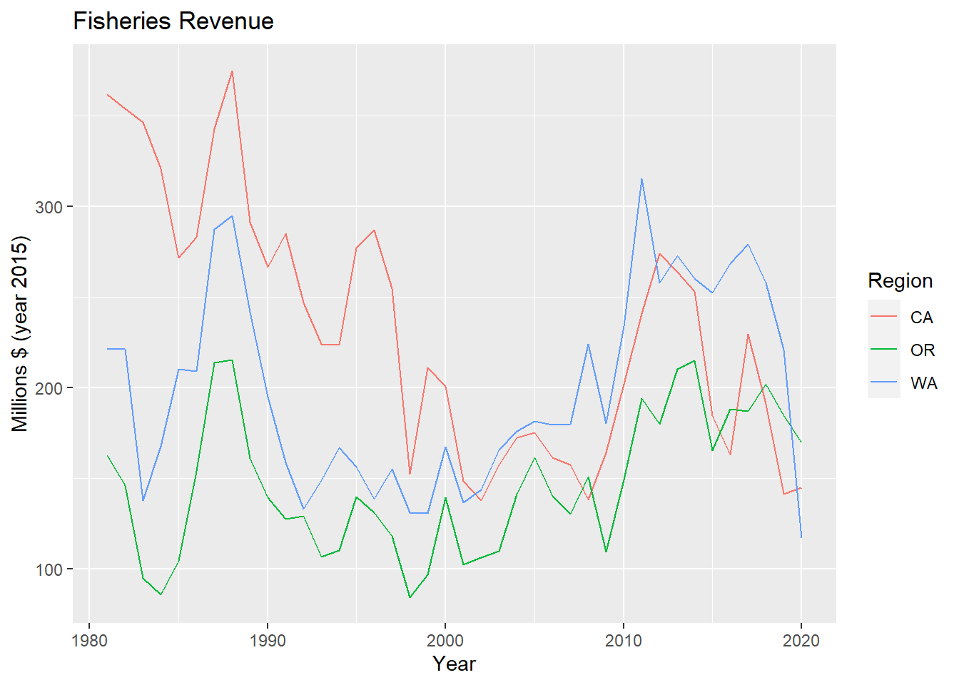
# show each region individually w/ facet_wrap
p_rgn +
facet_wrap(vars(region))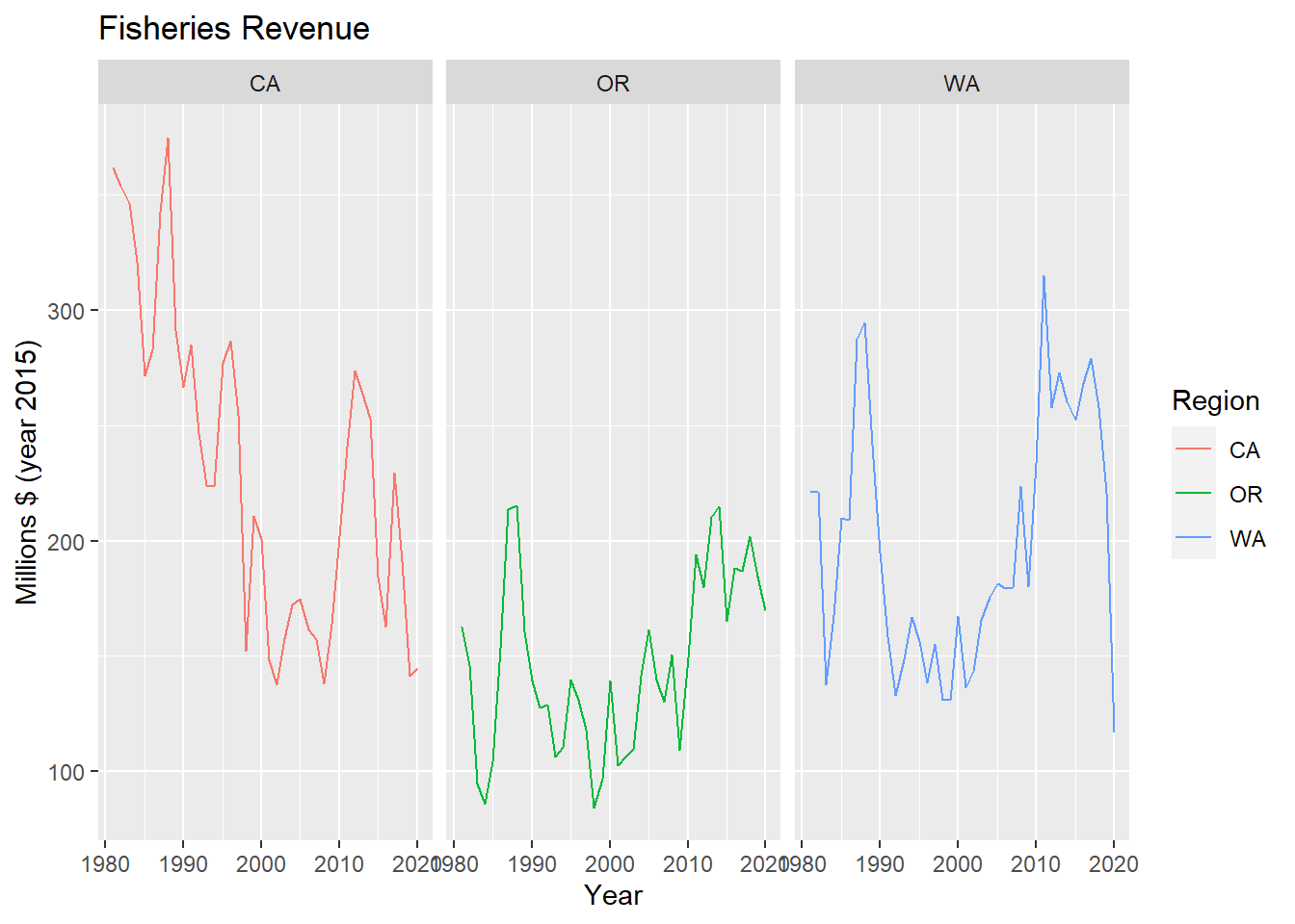 ## 3.3 Plot interactively with plotly or dygraphs ### 3.3.1 Make ggplot interactive with plotly::ggplotly()
# update all available packages
install.packages("plotly", repos = "http://cran.us.r-project.org")
## Error in install.packages : Updating loaded packagesplotly::ggplotly(p_rgn)